Area approximation from images is one very practical application of image processing. Probably one of its most basic applications is in remote land area approximation. Green’s Theorem and Morphological operations are the basic techniques involved in the appriximation. Using Scilab, SIP toolbox, and Paint, the area is estimated for regular, geometric shapes, as well as for some real samples taken from Googlemaps. The estimation was then verified by computing the theoretical area using the formulas for regular shapes, and areas for remote land area approximation was taken from the Web.
The first part of the activity deals with the basics; area approximation for regular shapes (circle, rectangle, and triangle). These regular shapes were drawn using Paint and saved as Bitmap files. They are drawn such that the inner part is white and the background is black. This is to enable using the follow command in Scilab which is a contour follower for binary images. It was observed that it really doesn’t work for other image types. Using the Scilab code shown below the image approximations were done for the abovementioned shapes.
C = imread(‘Circle.bmp’);
R = imread(‘Rectangle.bmp’);
T = imread(‘Triangle.bmp’);
[x_C,y_C]=follow(C);
[x_R,y_R]=follow(R);
[x_T,y_T]=follow(T);
a = length(x_C);
b = length(x_R);
c = length(x_T);
A_C = [];
A_R = [];
A_T = [];
for i=1:a-1
A_C(i) = x_C(i)*y_C(i+1)-y_C(i)*x_C(i+1);
end
for j=1:b-1
A_R(j) = x_R(j)*y_R(j+1)-y_R(j)*x_R(j+1);
end
for k=1:c-1
A_T(k) = x_T(k)*y_T(k+1)-y_T(k)*x_T(k+1);
end
Theo_Circle = %pi*((max(x_C)-min(x_C))/2)^2
Theo_Rectangle = (max(x_R)-min(x_R))*(max(y_R)-min(y_R))
Theo_Triangle = (max(x_T)-min(x_T))*(max(y_T)-min(y_T))*(1/2)
Area_Circle = sum(A_C)/2
Area_Rectangle = sum(A_R)/2
Area_Triangle = sum(A_T)/2
Percent_Error_Circle = abs(((Theo_Circle-Area_Circle)/(Theo_Circle))*100)
Percent_Error_Rectangle = abs(((Theo_Rectangle-Area_Rectangle)/(Theo_Rectangle))*100)
Percent_Error_Triangle = abs(((Theo_Triangle-Area_Triangle)/(Theo_Triangle))*100)
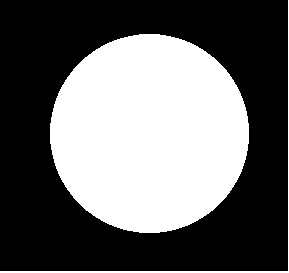
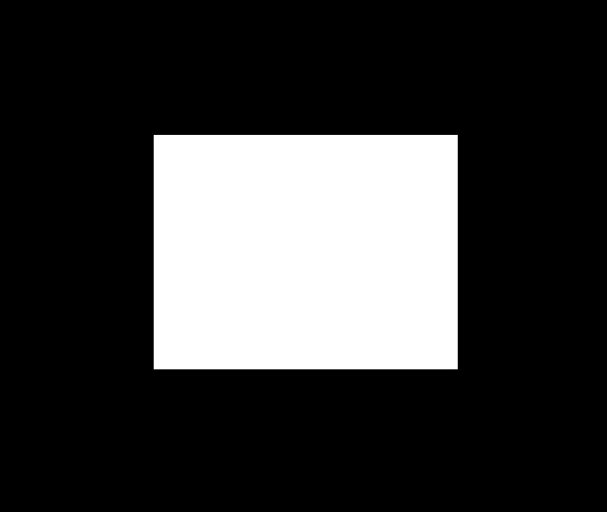
The figures used are shown below with informations on their respective area approximation.
Theoretical = 30790.75
Computed Area = 30760.5
Percentage Error = 0.0982425
The theoretical values is computed using the formula for the area of a circle, the radius used is just half the max-min pixel location.
Theoretical = 57814
Computed Area = 57644
Percentage Error = 0.2940464
The theoretical area is computed using the formula for finding the area of a rectangle. The dimensions used are the difference in the max and min pixel location for both x and y coordinates.
Theoretical = 36685
Computed Area = 36677
Percentage Error = 0.0218073
The theoretical area was computed using the formula for finding the triangle’s area which is . The base and the height were again taken from the difference of the max and the min pixel location.
It can be said that the estimation is effective from the small magnitudes of percentage errors. But this is only for the regular shaped image, how about area estimation on the real, complicated maps.
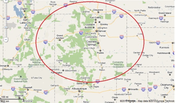
For more advanced applications, the same concept will be used for remote area approximation for the land areas of Colorado, USA, the Vatican City, and the Araneta Coliseum (this is in decreasing size). A print screen image was captured from the Googlemap and pasted on Paint. The borders for the specific area were defined by tracing with black lines/curves (this would introduce most of the errors that’s why a very tedious tracing must be employed). The ratio between the pixels and the physical measurement was computed using the given scale factor. Pixel locations were also obtained from Paint. The Region of Interest was then filled with white and the outer part with black. However, it should be noted that the obtained black and white image is not necessarily binary image, thus, conversion must be first made. Why make it binary? Since the Scilab command follow to be used is actually a counter follower for binary images.
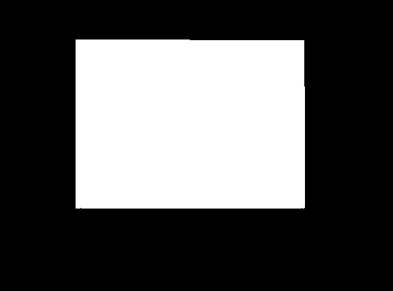
The validity of the approximation will be confirmed using their known land area. I will first engage in estimating Colorado’s land area because of all terrritories it has the simplest shape, simply rectangular.
Codes
Co = imread(‘Colorado.bmp’);
[x_Co,y_Co]=follow(Co);
d = length(x_Co);
A_Co = [];
for l=1:d-1
A_Co(l) = x_Co(l)*y_Co(l+1)-y_Co(l)*x_Co(l+1);
End
Theo_Colorado = 269837 //known value
Area_Colorado = sum(A_Co)/2
True_Area_Colorado = (Area_Colorado)*(3.36672) //km-pixel ratio
Percent_Error_Colorado = abs(((Theo_Colorado-True_Area_Colorado)/(Theo_Colorado))*100)
The result is given by
Theoretical = 269837
Computed Area = 36677
Computed Area multiplied with the ratio = 268578.4 (square kilometer)
Percentage Error = 0.4664280
From the Web, the area of Colorado is 269,837 square km. From my calculation the area in pixels is 36677. By using the scale factor from the ratio on Paint which is 109 pixels for every 200 km. The ratio in square km per pixel is 3.36672. This was multiplied to the computed area, and the result as shown has a percentage error of 0.4664280. It’s kinda effective, I think.
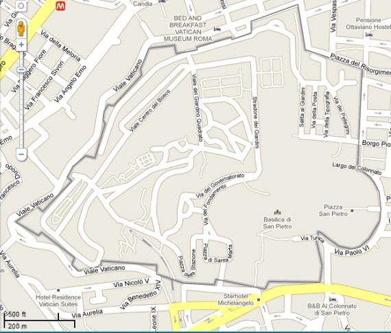
For more complex approximation, I will try estimating the area of the World’s smallest country, the Vatican City. So here’s it’s image from the Googlemap…
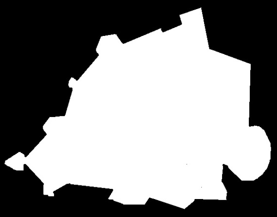
And here’s my binary image representation of it…
I have to say that my representation is not that exact since the map is so complicated . I have a hard time edge detecting… However, I will still try. So here’s my code;
V = imread(‘Vatican.bmp’);
[x_V,y_V]=follow(V);
e = length(x_V);
A_V = [];
for m=1:e-1
A_V(m) = x_V(m)*y_V(m+1)-y_V(m)*x_V(m+1);
end
Theo_Vatican = 440000 //known value
Area_Vatican = sum(A_V)/2
True_Area_Vatican = (Area_Vatican)*(3.2464897) //m-pixel ratio
Percent_Error_Vatican = abs(((Theo_Vatican-True_Area_Vatican)/(Theo_Vatican))*100)
The result is…
Theoretical = 440000 (square meter)
Computed Area = 470294.61
Percent Error = 6.8851396
Let me first give brief explanation before I bombard my own estimation with criticisms. The method I used here is similar to the previous method used. Here my square meter-pixel ratio is 3.2464897 as computed from the scale factor and from the information obtained by pixel locating in Paint.
Well, as expected I have a huge error for this one relative to my Colorado Area estimation. This just proves that it is harder to measure the area of complicated maps. I also have to blame my carelessness in edge detecting and tracing. But I can still say that, although my error is relatively big, for me it is still reliable.
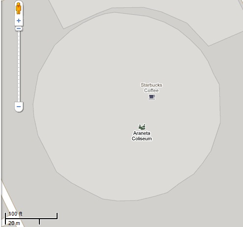
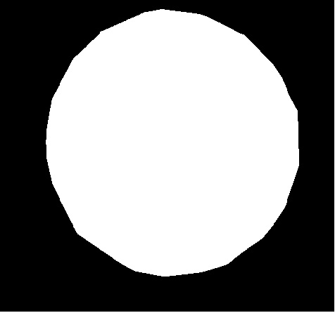
I will now try to estimate the area of a famous landmark. I chose the Araneta Coliseum, simply because I can find some necessary measurements of it from the Web. Following the same procedure as I have done before, a printscreen from Googlemaps is obtained and a binary image representation was made using the power of Paint!
Then it is now the Scilab’s job to do the computations. Here’s my code;
Ar= imread(‘Araneta.bmp’);
[x_Ar,y_Ar]=follow(Ar);
f = length(x_Ar);
A_Ar = [];
for n=1:f-1
A_Ar(n) = x_Ar(n)*y_Ar(n+1)-y_Ar(n)*x_Ar(n+1);
End
Theo_Araneta = %pi*(54)^2//108 is the dome diameter
Area_Araneta = sum(A_Ar)/2
True_Area_Araneta = (Area_Araneta)*(0.084016)//pixel-meter ratio
Percent_Error_Araneta = abs(((Theo_Araneta-True_Area_Araneta)/(Theo_Araneta))*100)
The result is given
Theoretical = 9160.8842
Computed Area = 9350.8548
Percentage Error = 2.0737147
Here my a priori knowledge of the Aranate Coliseum’s dimension is its diameter of 108 meters. So in my theoretical value I computed its area using that value. My pixel-meter ratio is 0.084016. 2% is indeed smaller than my previous attempt in estimating the area of the Vatican City. Of course it’s just because my image is much simpler.
As a conclusion, the method used is indeed reliable in area estimation. I am already happy with my maximum error of 6 %. My errors are definitely caused by the deformation of the original area when I made my binary image representations. (This can remedied by invoking much more OC-ness!). Another thing is on the pixel locating in computing for the pixel-to-physical quantity ratio. This is also prone to error given that the lines for the scale (scale bar?) are not just lines with single pixel.
There you go…I think I’ve done all the necessary things to do for this activity. I rate myself 10/10.
